EKF & Non-linear Least-Squares SLAM

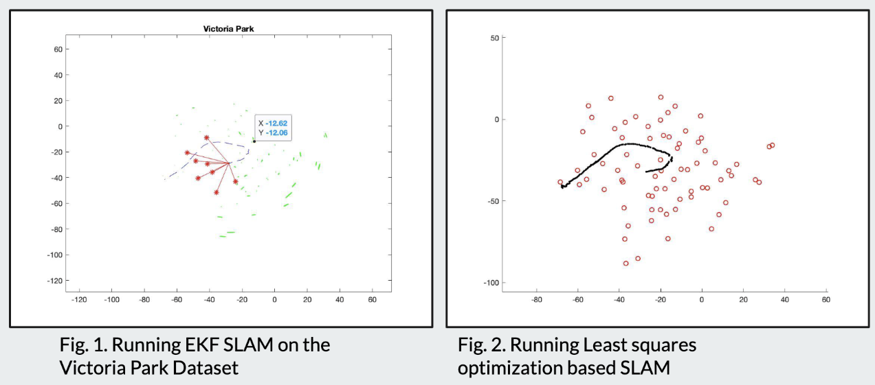
Implemented and compared two classical SLAM approaches on the Victoria Park Dataset: filter-based EKF-SLAM and optimization-based non-linear least-squares SLAM (Graph SLAM).

EKF-SLAM

The Extended Kalman Filter maintains a joint state vector of the robot pose and all landmark positions, updated incrementally as new observations arrive.

State Vector

The augmented state vector concatenates the robot pose \(\mathbf{x}_r = [x, y, \theta]^\top\) with \(N\) landmark positions:

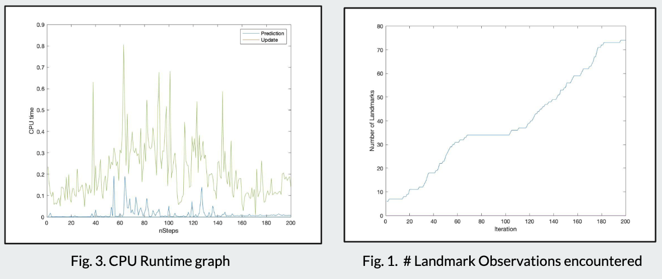
\[ \mathbf{x} = \begin{bmatrix} \mathbf{x}_r \\ \mathbf{m}_1 \\ \vdots \\ \mathbf{m}_N \end{bmatrix} \in \mathbb{R}^{3 + 2N} \]

Prediction Step

Given control input \(\mathbf{u}_t = [v_t, \omega_t]^\top\) (velocity and angular velocity), the motion model is:

\[ \mathbf{x}_{t+1} = f(\mathbf{x}_t, \mathbf{u}_t) = \begin{bmatrix} x_t + v_t \Delta t \cos(\theta_t) \\ y_t + v_t \Delta t \sin(\theta_t) \\ \theta_t + \omega_t \Delta t \end{bmatrix} \]

The covariance prediction uses the Jacobian \(\mathbf{F}_t\) of the motion model:

\[ \mathbf{P}_{t+1|t} = \mathbf{F}_t \, \mathbf{P}_{t|t} \, \mathbf{F}_t^\top + \mathbf{Q}_t \]

where \(\mathbf{Q}_t\) is the process noise covariance.

Update Step

For a range-bearing observation \(\mathbf{z} = [r, \phi]^\top\) of landmark \(j\):

\[ \mathbf{K}_t = \mathbf{P}_{t|t-1} \, \mathbf{H}_t^\top \left(\mathbf{H}_t \, \mathbf{P}_{t|t-1} \, \mathbf{H}_t^\top + \mathbf{R}_t\right)^{-1} \]

\[ \mathbf{x}_{t|t} = \mathbf{x}_{t|t-1} + \mathbf{K}_t \left(\mathbf{z}_t - h(\mathbf{x}_{t|t-1})\right) \]

where \(\mathbf{H}_t\) is the observation Jacobian, \(\mathbf{R}_t\) is the measurement noise, and \(\mathbf{K}_t\) is the Kalman gain.

Graph SLAM (Non-linear Least Squares)

The optimization-based approach constructs a factor graph where nodes represent robot poses and landmark positions, and edges encode odometry and observation constraints. The objective minimizes the sum of squared Mahalanobis distances:

\[ \mathbf{x}^* = \arg\min_{\mathbf{x}} \sum_{(i,j) \in \mathcal{C}} \left\| h_{ij}(\mathbf{x}_i, \mathbf{x}_j) - \mathbf{z}_{ij} \right\|^2_{\boldsymbol{\Omega}_{ij}} \]

where the weighted norm is \(\|\mathbf{e}\|^2_{\boldsymbol{\Omega}} = \mathbf{e}^\top \boldsymbol{\Omega} \, \mathbf{e}\) with information matrix \(\boldsymbol{\Omega}_{ij}\). This is solved iteratively using the Gauss-Newton algorithm, which linearizes the constraints at each step:

\[ \mathbf{H}^\top \boldsymbol{\Omega} \, \mathbf{H} \, \Delta \mathbf{x} = -\mathbf{H}^\top \boldsymbol{\Omega} \, \mathbf{e} \]

Comparison

Aspect	EKF-SLAM	Graph SLAM
Complexity per step	\(\mathcal{O}(N^2)\)	\(\mathcal{O}(N)\) amortized
Memory	Dense covariance \(\mathcal{O}(N^2)\)	Sparse factors \(\mathcal{O}(N)\)
Consistency	Approximation errors accumulate	Global optimization, more consistent
Loop closure	Difficult to incorporate	Natural via graph edges
Linearization	Single linearization point	Re-linearization at each iteration